I'm interested in all aspects of forward-modelling and inversion of geophysical data. Below are some specific topics I'm working on now or have done so in the past.
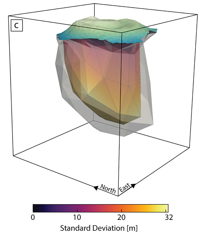
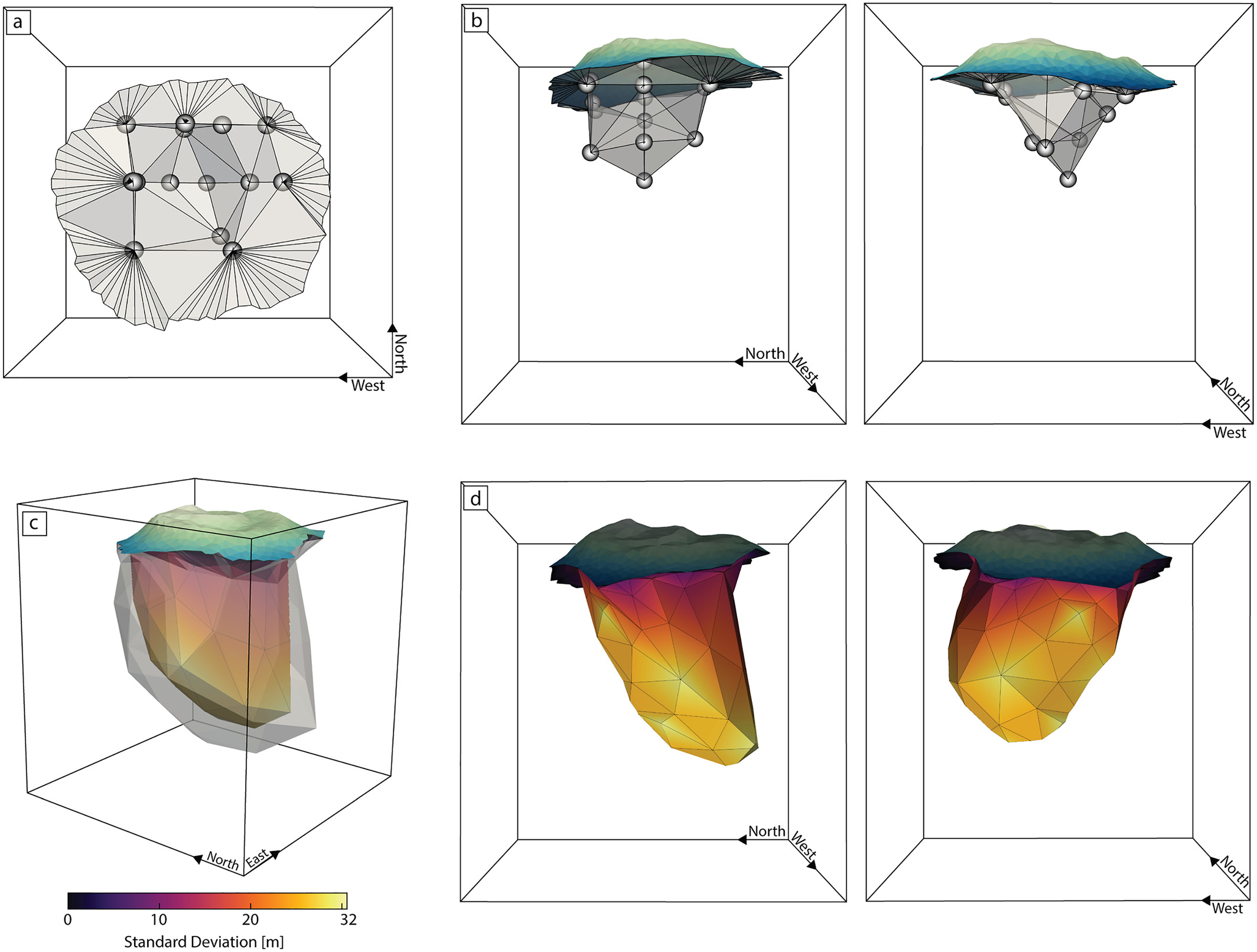
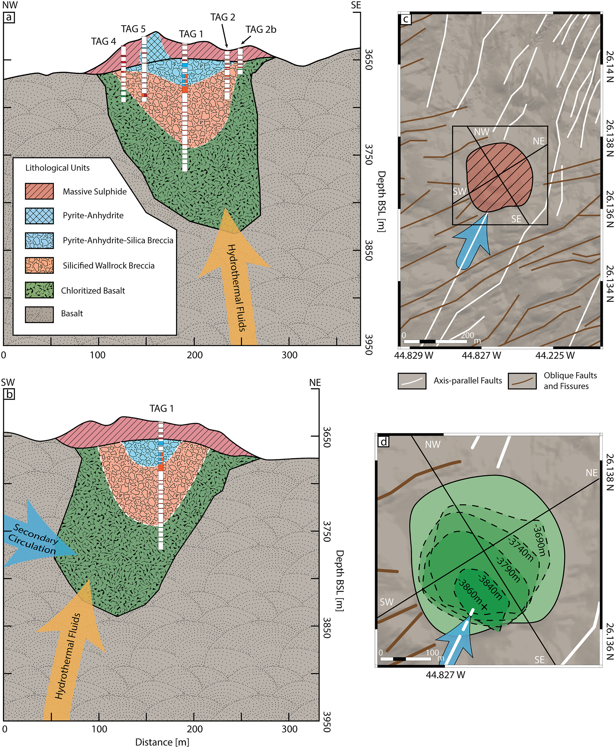
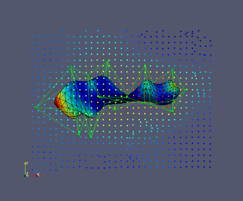
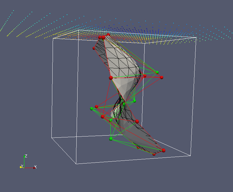
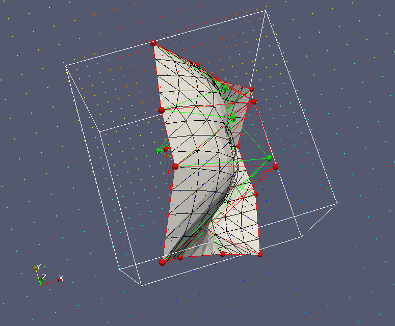
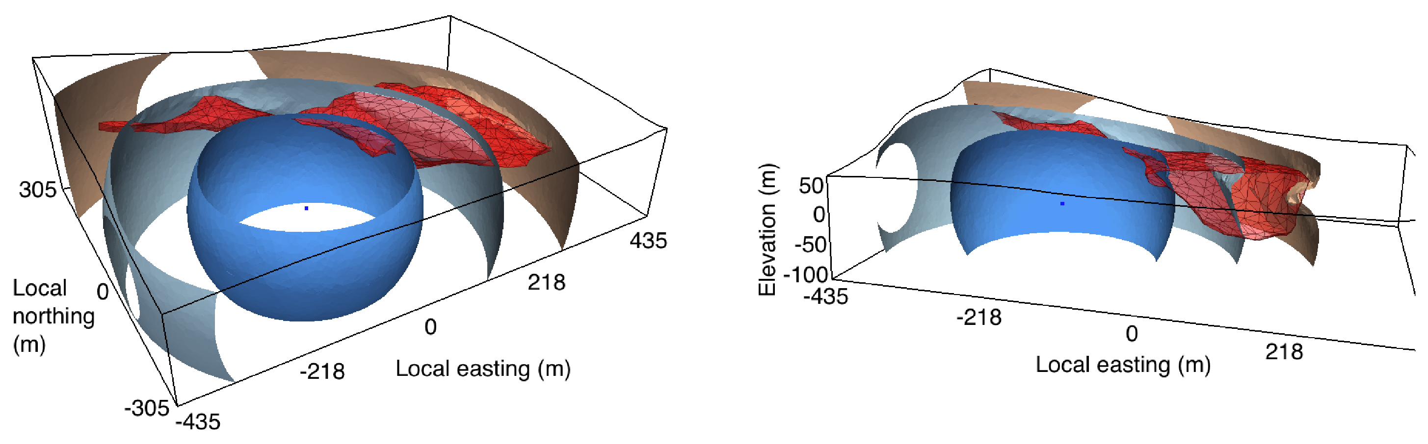
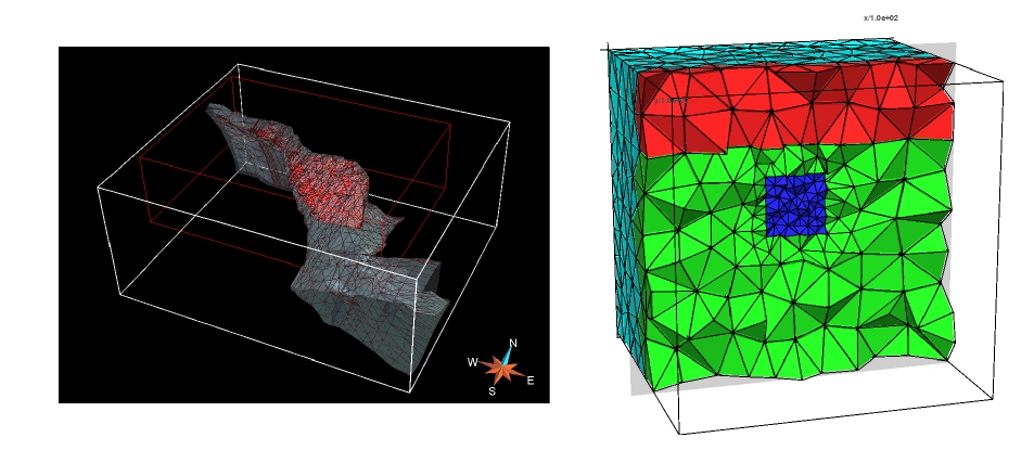
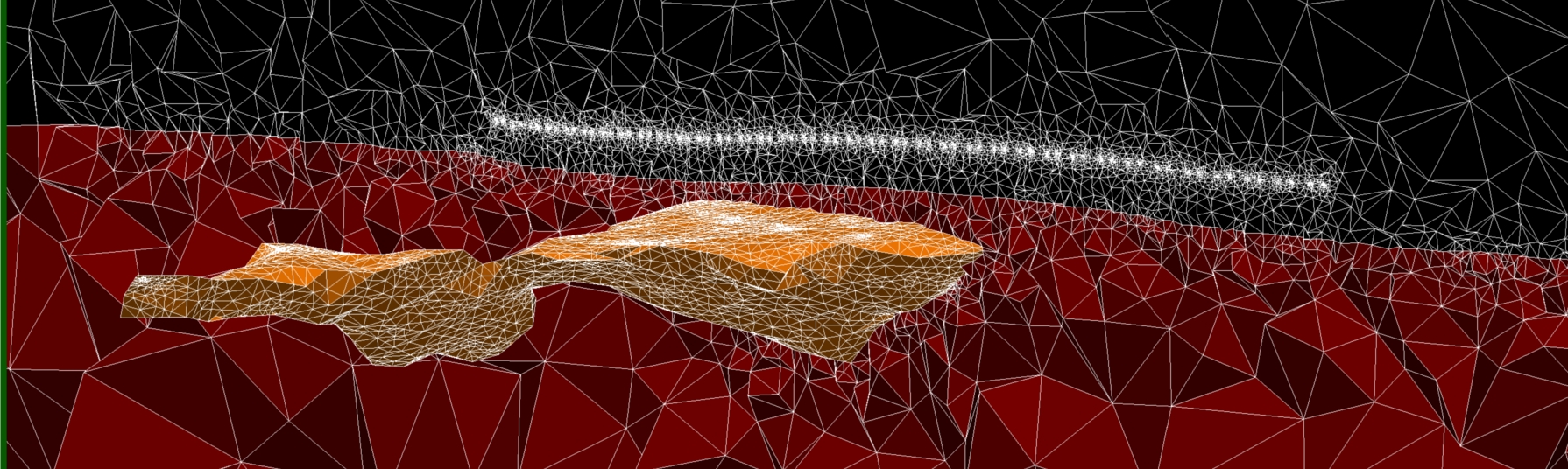
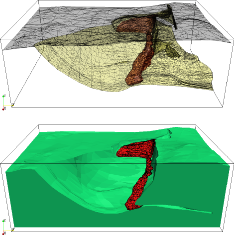
Surface Geometry Inversion (SGI): We are continuing to develop our "surface geometry inversion" (SGI) approach. (Earlier work is also mentioned below.) This approach works with a wireframe model of the Earth's subsurface. The wireframe surfacess (typically surfaces made up of tessellations of triangular facets, as that's the most flexible and general) are the contacts between the different geological units. These wireframe surfaces are moved around during the inversion process. We are using Genetic Algoritms as the global optimization method, with a follow-on Markov chain Monte Carlo sampling procedure to get uncertainties in the optimal locations of the wireframe interfaces. So far Peter and Chris Galley have implemented and used SGI for gravity and magnetics, and Xushan Lu is implementing SGI for time-domain EM and DC resistivity. More on this below.
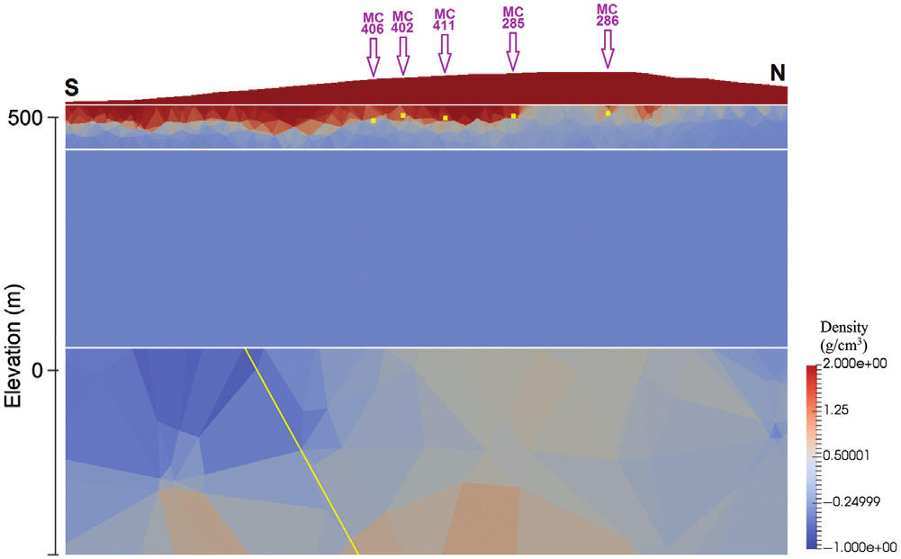
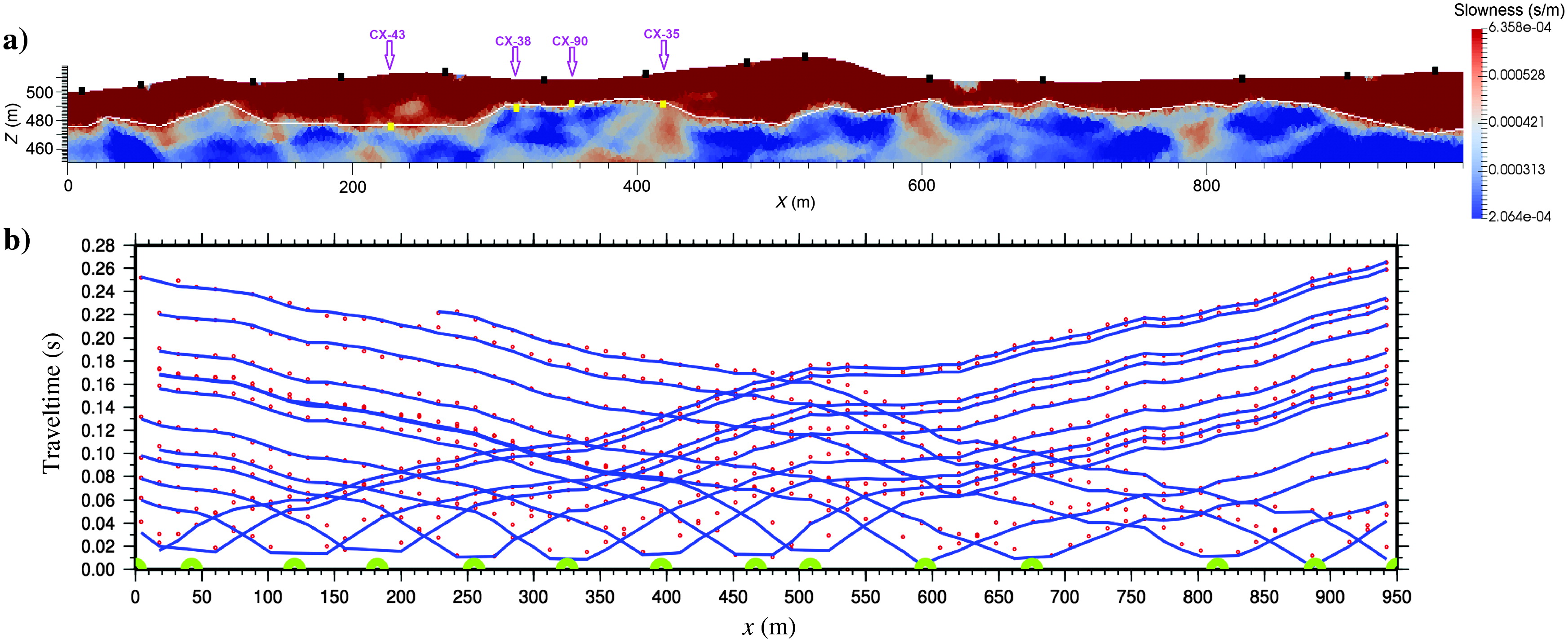
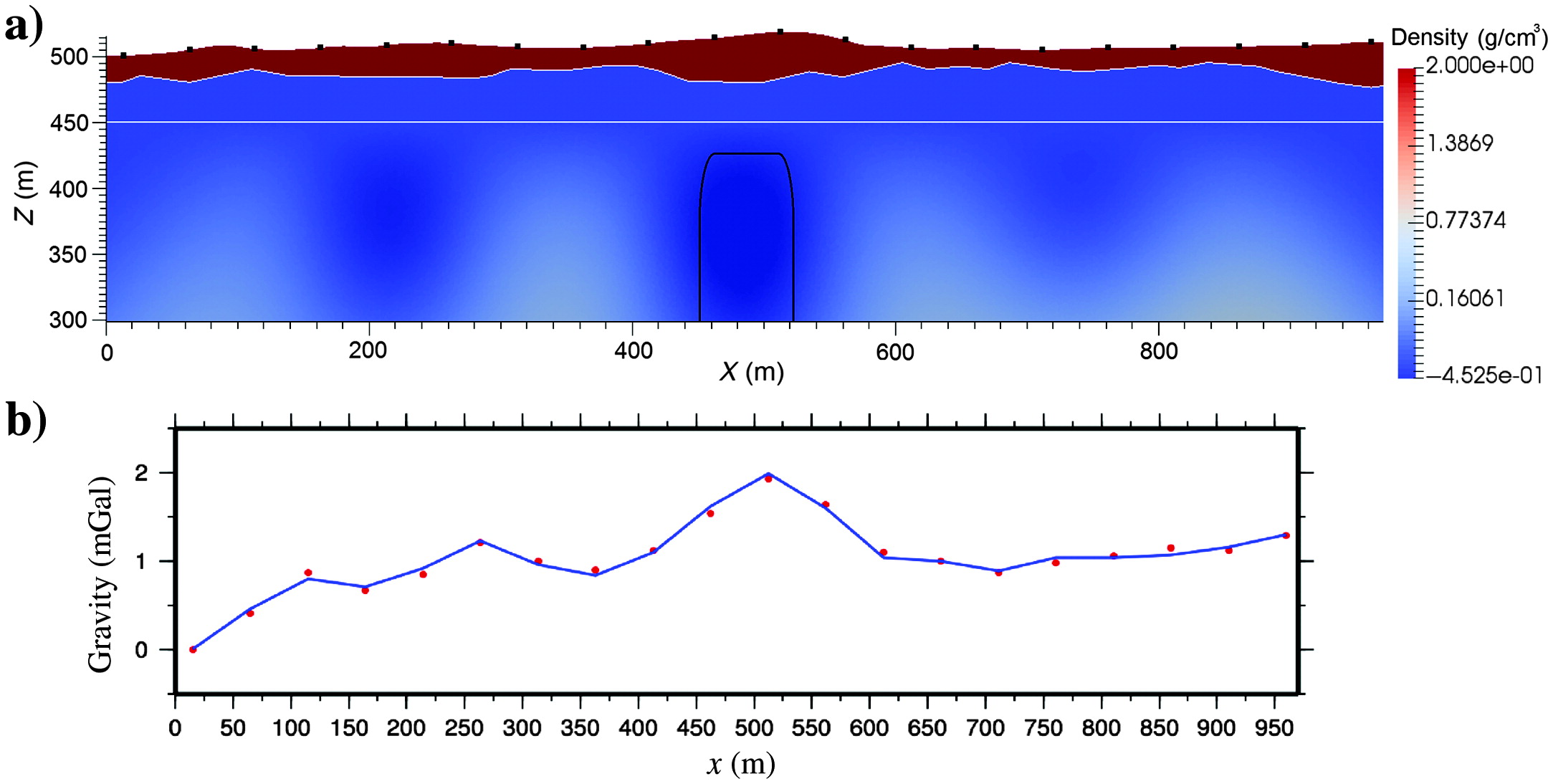
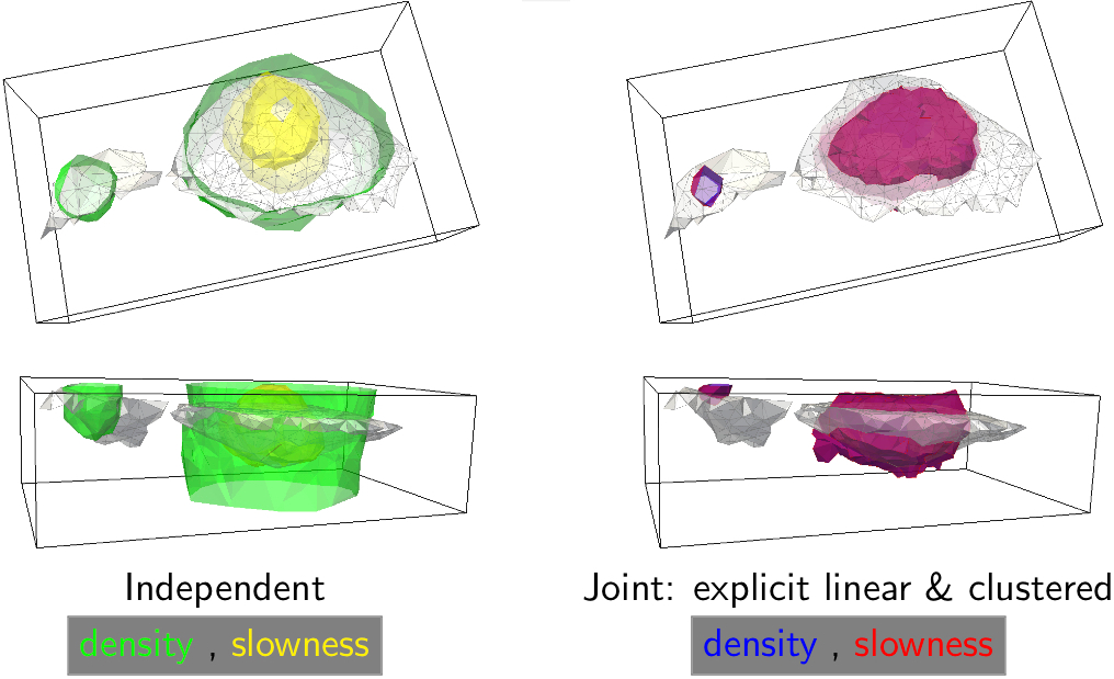
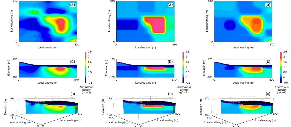
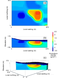
More joint inversion, and clustering inversion: Mehrdad Darijani, for his PhD project, applied Peter's joint and clustering inversion codes (gravity, magnetics, seismic travel-time) to data from the Athabasca Basin as part of the CMIC "Footprints" project. The challenge was to determine the thickness of the quaternary sediments, and to take this into account when modelling and inverting the gravity data, with the ultimate aim being to get information about possible alteration zones within the sandstones (which could be indicators of uranium deposits). The variable thickness of the quaternary sediments nicely obfuscates any gravity signal coming from alteration deeper in the sandstones. Mehrdad tried various combinations of data---seismic refraction, magnetic, gravity---and various inversion approaches---gravity inversion constrained by results of seismic inversion, joint gravity and magnetic inversion, joint gravity and seismics, regular sum-of-squares and clustering---to see if any alteration in the sanstones could be made out. More on this below.
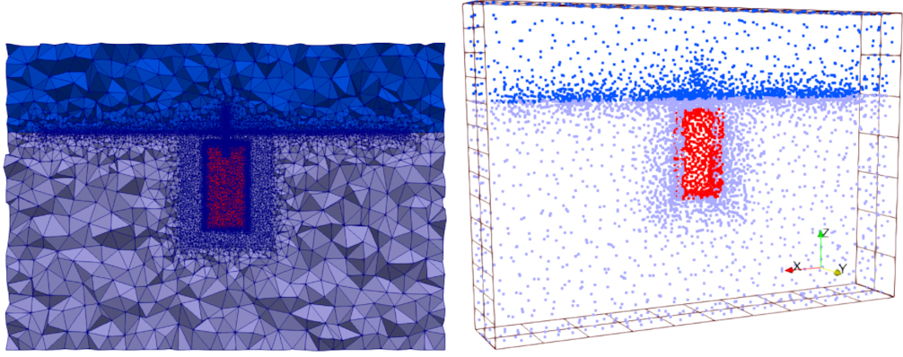
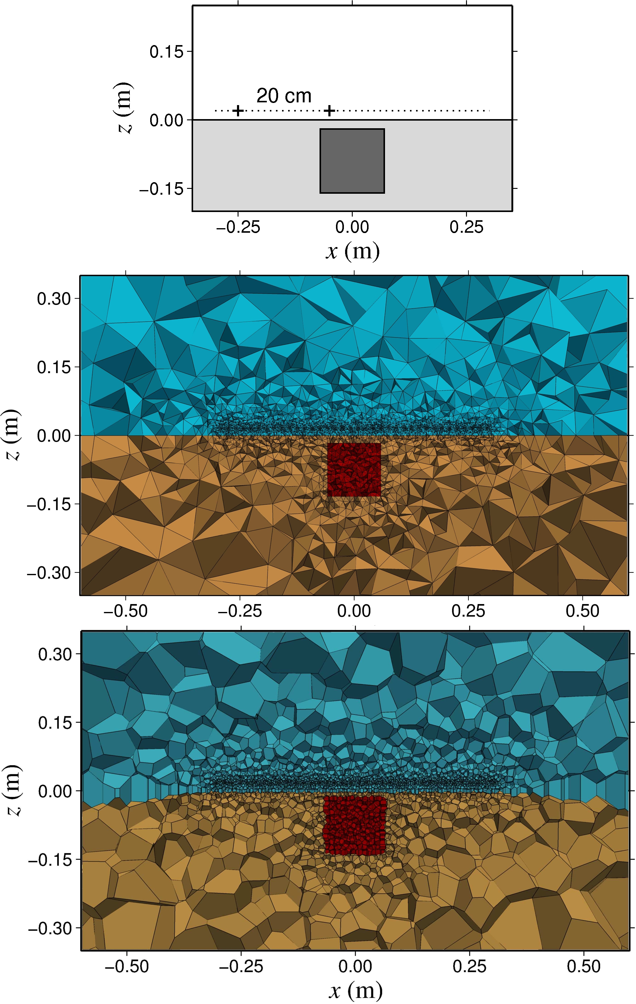
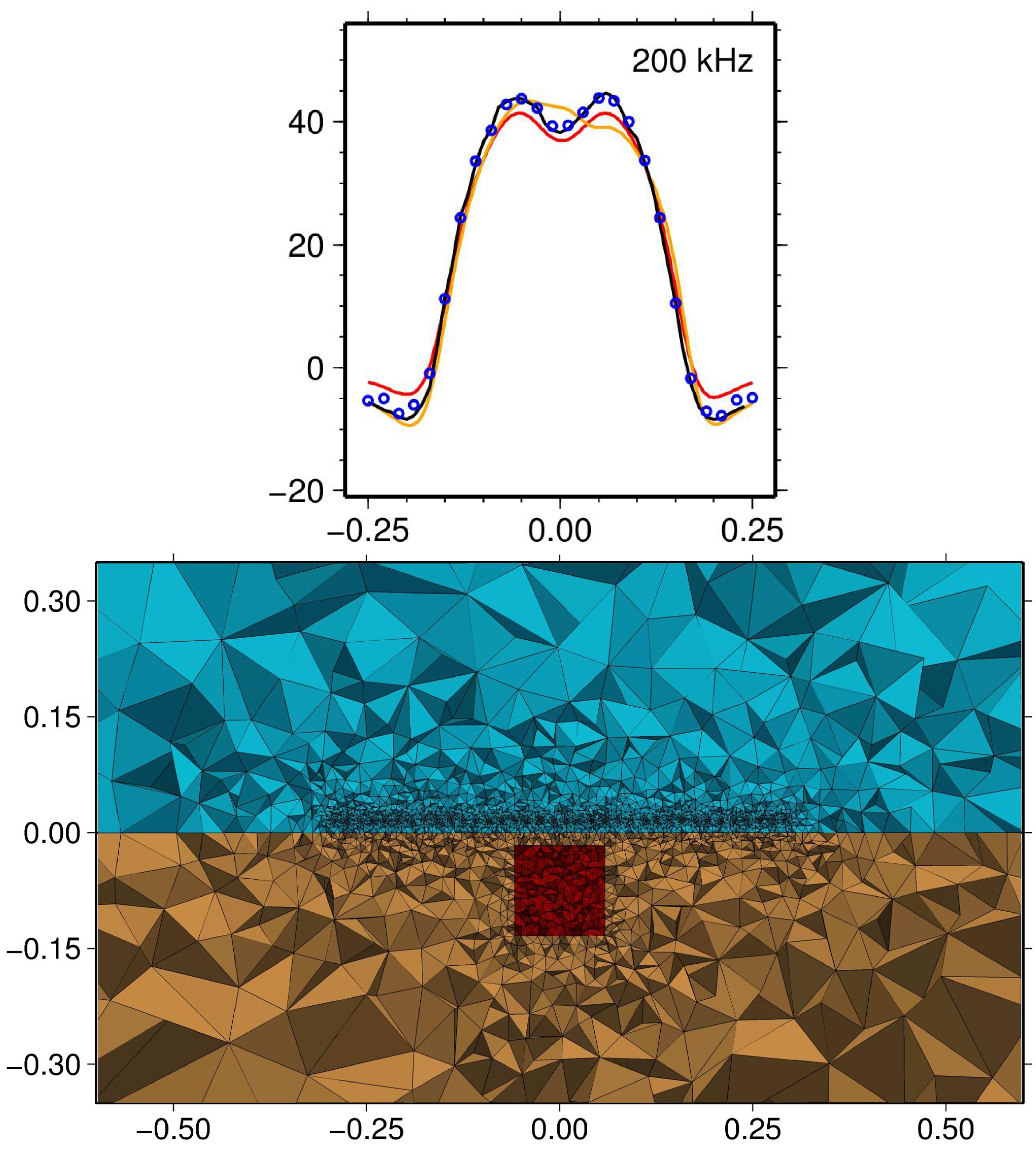
Meshfree forward modelling: Unstructured tetrahedral meshes are very flexible and powerful for discretizing volumes between arbitrary, complicated surfaces (topography!). However, for certain forward-modelling problems such as finite-element solutions to the EM equations, the "quality" of the mesh, i.e., how *not* long and pointy the tetrahedral cells are, is important. However, for models with lots of complicated surfaces, it can be hard to generate a high quality tetrahedral mesh. Wouldn't it be great if we could have one mesh (unstructured tetrahedral mesh) for parameterizing the Earth model, and a separate, distinct mesh (or simply a cloud of nodes!) for the numerical solution of the partial differential equation? Jianbo Long investigated this for his PhD, implementing meshfree meshes for gravity and for EM. More on this below.
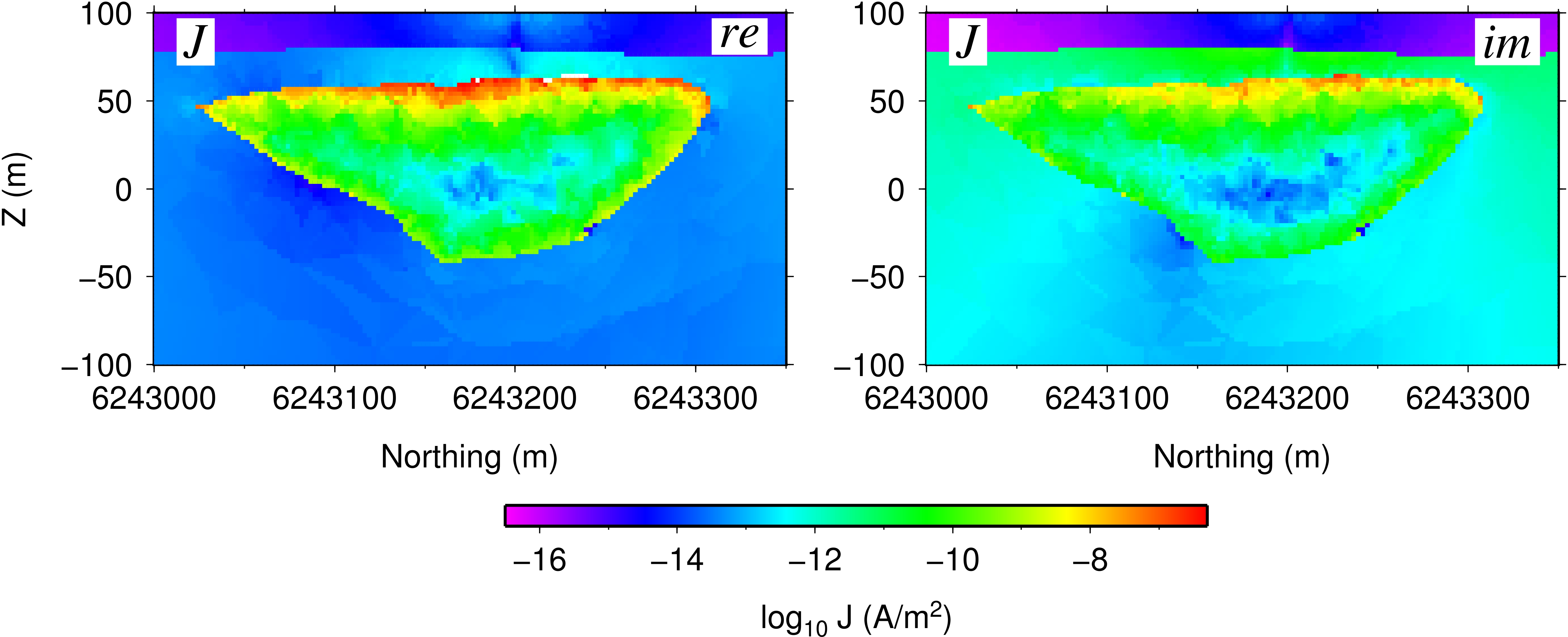
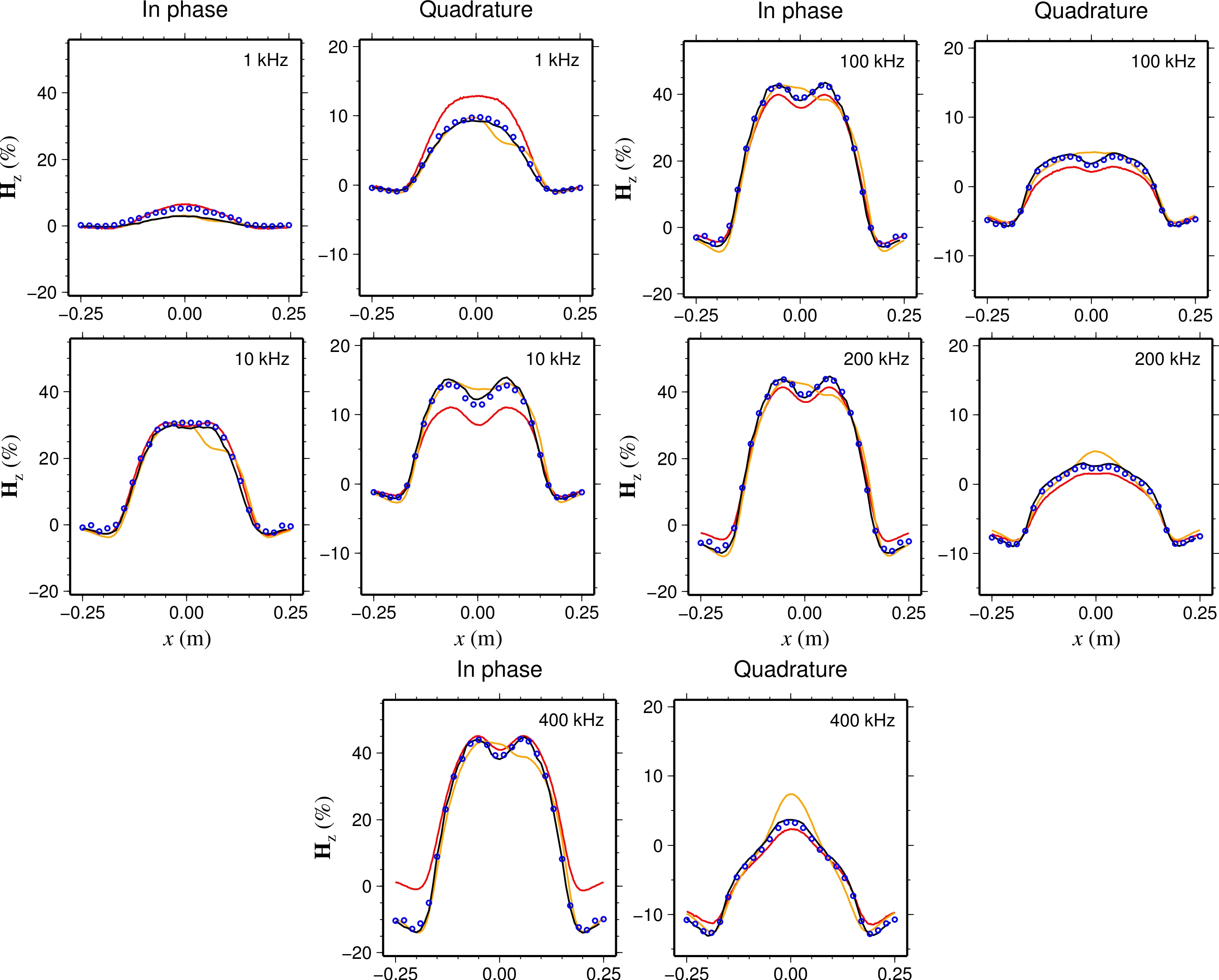
3-D EM forward modelling for real-life Earth models: We have successfully applied our various 3-D EM forward-modelling codes to a number of real-life Earth models, including high conductivity contrast mineral exploration scenarios and marine CSEM hydrocarbon exploration scenarios. Between my two post-docs, Masoud Ansari and Hormoz Jahandari, and Dr. Jianhui Li who visited us last year, we have finite-element and finite-volume codes both for E-field and vector-scalar potential formulations. More on this below.
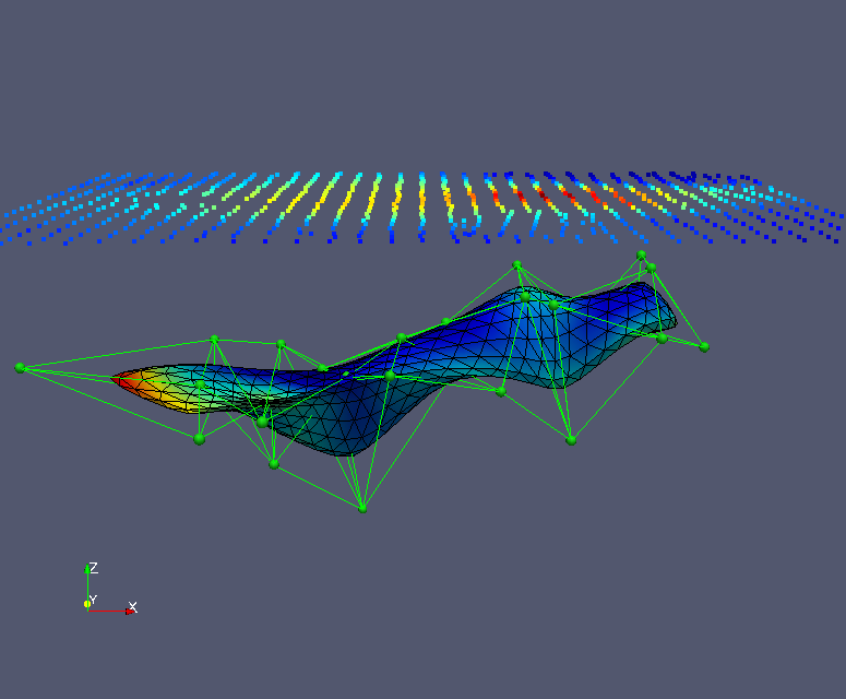
Surface-based inversion: We (well Peter Lelièvre is!) are investigating inversion methods that can work with the surfaces in a wireframe Earth model. The goal is to have the geophysical inversion work on exactly the same Earth model that the geologists are working with. One approach is to parameterize the surfaces using a small number of control nodes with subsequent surface subdivision, and then to invert for the locations of these nodes using a global optimization technique. For a little more on this please see below.
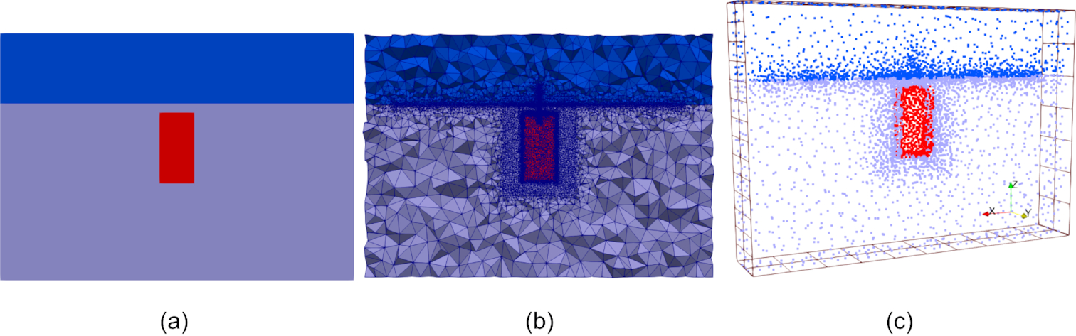
3-D EM forward modelling on unstructured meshes: Two of my PhD students, Masoud Ansari and Hormoz Jahandari, have developed 3-D controlled-source EM forward modelling methods for Earth models parameterized in terms of unstructured tetrahedral meshes. Masoud has implemented a finite-element approach with the electric field decomposed into vector and scalar potentials. This enables the relative importance of the inductive and galvanic contributions to the electromagnetic fields generated in the Earth to be investigated. Hormoz has developed a finite-volume approach that essentially corresponds to a staggered grid formulation for tetrahedral meshes. Both Masoud and Hormoz use total field formulations so that sources on arbitrary topography can be considered. More on this below.
Different discretizations of the subsurface, continued; computational geophysics on unstructured grids: We have been working on computational methods for unstructured grids for a couple of years now. (Initial thoughts are preserved below.) We've been working through most of the data types one would want. So far we've developed code for modelling gravity, gravity gradient, magnetic, seismic travel-time, DC resistivity, and electromagnetic data. This is using finite element and finite volume methods on tetrahedral and Voronoï grids for the potential field methods and EM, and an implementation of a fast marching method on tetrahedral grids for seismic travel times. We currently have inversion code for gravity, gravity gradiometry, magnetic and seismic travel-time data (including joint inversion - see the next topic); inversion code for EM may follow. A few more specifics on all this below.
Joint inversion: Inverting two or more data-sets for some kind of common Earth model is arguably the most active research area in geophysical inversion at the moment. I am very lucky to be working with Dr. Peter Lelièvre, an NSERC Post-Doctoral Fellow in my group. (Peter's home page is here.) Peter has been working on the joint inversion of seismic travel-time and gravity data. Our current strategy is to optimize an objective function that comprises the usual measures of data misfit and model structure for the individual data-sets and physical properties plus a measure of model similarity. We are using a combination of one or more of the following for the measure of similarity: explicit analytic relationship, implicit analytic relationship, statistical relationship. More below.
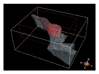
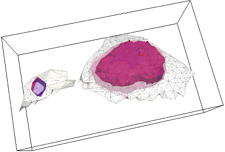
Different discretizations of the subsurface: The usual way at the moment for we geophysicists to discretize the Earth, and thus obtain a model of the spatial variation of some physical property in the subsurface, is to use a regular rectangular grid. This is by far the easiest kind of mesh to deal with, especially in terms of the information required to keep track of where all the cells and nodes are in the model. However, this is perhaps not the best kind of mesh for representing the possible geological features in the Earth. Wouldn't it be better to have a mesh that could follow known (or projected) interfaces such as faults and contacts between rock units? More below. (No, the picture to the left, which is of the wire-frame geological model of the Ovoid deposit at Voisey's Bay, Labrador, is not squint.)
Blocky models in minimum-structure inversions: Minimum-structure inversions (in which the model is finely parameterized, and a measure of model complicatedness is minimized along with a measure of data-misfit) have many good points, notably reliability and robustness. Typical, traditional implementations use an l2, or sum-of-squares, measure for the complicatedness. This is why the models which are produced have their characteristic fuzzy, smeared-out appearance. If an l1 measure is used instead, models with sharp interfaces between zones of uniform physical parameter can be constructed. Also, if diagonal finite-differences are explicitly included in the measure of model structure, angled interfaces can be generated in the model. (If only finite differences in the x-, y- and z-directions are included, only horizontal and vertical interfaces are generated.) More below.
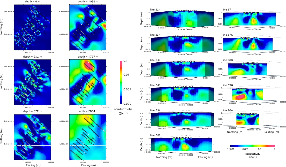
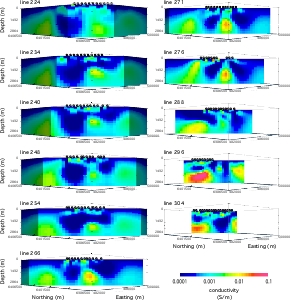 3-D magnetotelluric inversion:
While at
UBC-GIF,
I wrote the MT-relevant bits of the 3-D MT inversion program MT3Dinv.
This program shares components with the controlled-source EM forward-modelling
and inversion programs EH3D and EH3Dinv that were developed by
Eldad Haber,
Roman Shekhtman and Doug Oldenburg.
All these programs came out of the
IMAGE
consortium research project at UBC-GIF.
I have since been testing MT3Dinv on various data-sets.
For example, in conjunction with Jim Craven
(GSC, Ottawa),
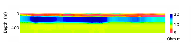
I have inverted the AMT data-set from over the McArthur River uranium mine
in Saskatchewan.
The results are (quite?) good.
But 3-D inversion of multi-frequency EM data is still so computationally expensive
that suitably discretized models, and appropriately converged iterative linearized
inversion procedures, are still elusive.
More below.
3-D magnetotelluric inversion:
While at
UBC-GIF,
I wrote the MT-relevant bits of the 3-D MT inversion program MT3Dinv.
This program shares components with the controlled-source EM forward-modelling
and inversion programs EH3D and EH3Dinv that were developed by
Eldad Haber,
Roman Shekhtman and Doug Oldenburg.
All these programs came out of the
IMAGE
consortium research project at UBC-GIF.
I have since been testing MT3Dinv on various data-sets.
For example, in conjunction with Jim Craven
(GSC, Ottawa),
I have inverted the AMT data-set from over the McArthur River uranium mine
in Saskatchewan.
The results are (quite?) good.
But 3-D inversion of multi-frequency EM data is still so computationally expensive
that suitably discretized models, and appropriately converged iterative linearized
inversion procedures, are still elusive.
More below.
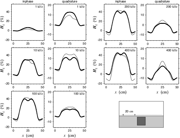
Integral equation solution for large contrasts: Traditional implementations of the integral equation solution to the geophysical electromagnetic forward-modelling problem fail for large conductivity contrasts. I have developed an implementation that does not have this limitation. It has been tested against results from physical scale modelling performed by Ken Duckworth formerly at the University of Calgary. More below.
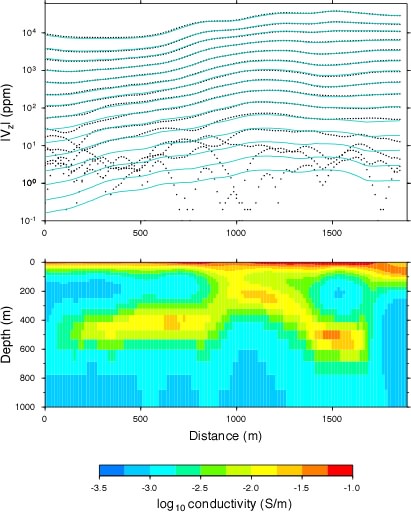
 Program EM1DTM:
This is the sister program to
EM1DFM,
which I wrote a few years ago while at
UBC-GIF.
(EM1DFM is available for commercial and academic licensing: see the relevant UBC-GIF
page.)
Program EM1DTM is for time-domain EM data, particularly lines or grids of many
soundings (that is, what one gets from airborne surveys).
Like EM1DFM, nifty things such as the GCV or L-curve criteria can be used to
automatically estimate the trade-off parameter.
Unlike EM1DFM though, EM1DTM includes general measures, and so can produce blocky,
piecewise-constant models if desired.
More below.
Program EM1DTM:
This is the sister program to
EM1DFM,
which I wrote a few years ago while at
UBC-GIF.
(EM1DFM is available for commercial and academic licensing: see the relevant UBC-GIF
page.)
Program EM1DTM is for time-domain EM data, particularly lines or grids of many
soundings (that is, what one gets from airborne surveys).
Like EM1DFM, nifty things such as the GCV or L-curve criteria can be used to
automatically estimate the trade-off parameter.
Unlike EM1DFM though, EM1DTM includes general measures, and so can produce blocky,
piecewise-constant models if desired.
More below.